Get Standardized Marginal Score Statistics — getZ_marg

Calculates the standardized marginal score statistics for each variant under a generalized linear model framework. This is the foundation function for all GLOW tests, providing the score statistics and their correlation structure.

For continuous traits, there is an option to use t-statistics from the lm() function of Y on each column of G and X. This t-statistic is close to the null-model defined marginal score statistics but not exactly the same, partially due to different ways of estimating the error variance.

getZ_marg_score(
  G,
  X = NULL,
  Y = NULL,
  trait = "binary",
  null_model = NULL,
  use_lm_t = FALSE,
  use_cpp = FALSE
)

Arguments

G: A numeric matrix of genotypes (n x p), where n is the number of individuals and p is the number of SNPs. Missing values (NA) are not allowed.
X: A numeric matrix of covariates (n x k), where k is the number of covariates. Required if null_model = NULL. Ignored if null_model is provided.
Y: A numeric vector of response variable (length n). For binary traits, must be coded as 0/1. For continuous traits, any numeric values are allowed. Required if null_model = NULL. Ignored if null_model is provided.
trait: Character string indicating trait type. Must be either "binary" (logistic regression) or "continuous" (linear regression). Default is "binary". Ignored if null_model is provided (trait is extracted from null_model).
null_model: Optional. A null_model object from fit_null_model(). If provided, the function reuses the pre-computed null model, which can improve performance for repeated calls with different SNP sets. When null_model is provided, X, Y, and trait are ignored. Default is NULL (standard mode - fit null model from X and Y).
use_lm_t: Logical. For continuous traits, whether to use t-statistics from lm() function as Z-scores. If FALSE (default), uses null-model defined Z-scores. Ignored for binary traits.
use_cpp: Logical. Whether to use C++ implementation for GHG matrix computation. Default is FALSE (use R). The C++ version may be faster on some platforms (Linux with standard BLAS), but is not necessarily so on Apple Silicon due to highly optimized ARM64 BLAS. Set to TRUE to force C++ usage for portability testing.

Value

A list with the following components:

Zscores: Numeric vector (length p) of standardized marginal score statistics (Z-scores) for each variant
scores: Numeric vector (length p) of marginal score statistics for each variant. For the standard method, $Z_j = S_j / (\sqrt{M_{s,jj}} \cdot s_0)$ (exact relationship). Compare with the SPA method where Z-scores are derived from SPA-adjusted p-values.
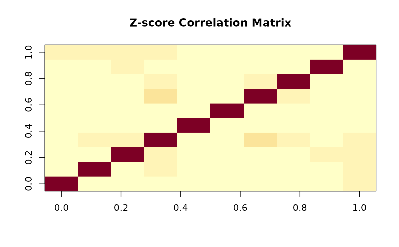
M_Z: Numeric matrix (p x p) giving the correlation matrix of Z-scores when effects are fixed (including H0), given X and G fixed
M_s: Numeric matrix (p x p) giving the covariance matrix of score statistics when effects are fixed (including H0), given X and G fixed
s0: Numeric scalar giving the estimated dispersion parameter. For binary traits, s0 = 1. For continuous traits, s0 is the residual standard deviation under the null model

Details

The function implements the following algorithm:

For Binary Traits (Logistic Regression):

Fit null model: $\text{logit}(P(Y=1)) = X\beta$
Compute fitted probabilities: $Y_0 = \hat{P}(Y=1|X)$
Define weighted design matrix: $\tilde{X} = \sqrt{Y_0(1-Y_0)} \cdot X$
Compute projection: $H^{1/2} = \tilde{X}({\tilde{X}}'\tilde{X})^{-1/2}$
Define weighted genotype matrix: $\tilde{G} = \sqrt{Y_0(1-Y_0)} \cdot G$
Compute score variance: $M_s = {\tilde{G}}'{\tilde{G}} - {\tilde{G}}'H^{1/2}{H^{1/2}}'{\tilde{G}}$
Compute score statistics: $S = G'(Y - Y_0)$
Compute Z-scores: $Z_j = S_j / \sqrt{M_{s,jj}}$
Set dispersion: $s_0 = 1$

For Continuous Traits (Linear Regression):

Fit null model: $Y = X\beta + \epsilon$
Compute projection: $H^{1/2} = X(X'X)^{-1/2}$
Compute score variance: $M_s = G'G - G'H^{1/2}{H^{1/2}}'G$
Obtain residuals: $r = Y - X\hat{\beta}$
Estimate dispersion: $s_0 = \text{SD}(r)$
Compute score statistics: $S = G'r / s_0$
If use_lm_t = TRUE: Extract t-statistics from marginal regressions
If use_lm_t = FALSE: Compute Z-scores as $Z_j = S_j / \sqrt{M_{s,jj}}$

The correlation matrix $M_Z$ is obtained by standardizing $M_s$: $$M_Z = \text{cor}(M_s)$$

Mathematical Properties:

The Z-scores are asymptotically standard normal under the null hypothesis
$M_Z$ represents the correlation of Z-scores when effects are fixed (including H0)
$M_s$ is the covariance matrix of score statistics under fixed effects
The function properly accounts for correlation induced by covariates through projection

Computational Complexity:

Time: $O(n \cdot p \cdot k + p \cdot k^2)$ where n = sample size, p = number of SNPs, k = number of covariates
Space: $O(p^2 + n \cdot p + n \cdot k)$

References

Zhang, H., Liu, M., Landers, J. E., and Wu, Z. (2026). Integrated weighted association test with application to genetic association studies. The Annals of Applied Statistics, 20(3), 2074-2097. doi:10.1214/26-AOAS2223

Examples

# Example 1: Continuous trait with null-model Z-scores (default)
set.seed(123)
n <- 500
p <- 10
# Generate genotypes with varying MAF
G <- matrix(0, n, p)
for (j in 1:p) {
  maf <- 0.05 * j / p  # MAF from 0.005 to 0.05
  G[, j] <- rbinom(n, 2, maf)
}
# Covariates: intercept will be added automatically
X <- matrix(rnorm(n * 2), n, 2)
Y <- rnorm(n)  # Continuous trait
result_cont <- getZ_marg_score(G, X, Y, trait = "continuous")
head(result_cont$Zscores)
#> [1]  0.73178942 -0.42718517  0.04708312 -1.32524883 -1.22966548  0.10964021

# Example 2: Continuous trait with lm() t-statistics
result_lm_t <- getZ_marg_score(G, X, Y, trait = "continuous", use_lm_t = TRUE)
head(result_lm_t$Zscores)
#> [1]  0.72997814 -0.42597701  0.04694148 -1.32359042 -1.22782521  0.10931145

# Example 3: Binary trait
Y_binary <- sample(c(0, 1), n, replace = TRUE)
result_binary <- getZ_marg_score(G, X, Y_binary, trait = "binary")
head(result_binary$Zscores)
#> [1]  0.6116281 -0.1778623  0.1890274 -1.1363778  1.2678918 -1.4360598
result_binary$s0  # Should be 1 for binary traits
#> [1] 1

# Example 4: Examine correlation structure
result <- getZ_marg_score(G, X, Y, trait = "continuous")
image(result$M_Z, main = "Z-score Correlation Matrix")


# Example 5: Optimized workflow for multiple SNP sets (RECOMMENDED FOR GWAS)
# Create multiple gene sets
gene_sets <- lapply(1:100, function(i) {
  matrix(rbinom(n * 5, 2, runif(1, 0.01, 0.1)), n, 5)
})

# Step 1: Fit null model once
null_obj <- fit_null_model(X, Y_binary, trait = "binary")

# Step 2: Reuse for all gene sets (much faster!)
results_optimized <- lapply(gene_sets, function(G_gene) {
  getZ_marg_score(G_gene, null_model = null_obj)
})

# This is ~10-100x faster than refitting null model for each gene set